
If you’re interested in experimenting yourself with the topics in this post, you may want to check out the code I used to generate all the graphs and stats in the accompanying jupyter notebook.
Introduction#
Reasoning about high dimensional spaces using geometric intuition is hard, our brains just aren’t build to imagine such spaces. My aim in this article is to give a stastical intuition as to why the angle between two random vectors becomes increasingly likely to be close to 90 degrees, in other words the vectors become more orthogonal, as you increase the number of dimensions of those vectors.
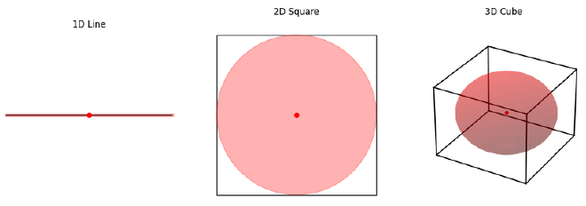
In my opinion, the sparsity in terms of angles is a little less intuitive than sparsity in terms of distance between points: I can imagine that as you go from a line, to a square, to a cube, the amount of space (e.g. volume) contained within the object is increasing a lot, so it makes sense that points in high dimensional spaces tend to be further apart.
However, the sparsity in terms of angles is less obvious, at least to me. When I imagine putting two random points in a square, and then a cube, it doesn’t feel like the distribution of the angle between the points (and the origin) is trending in any obvious direction. This is where viewing the problem statistically can be useful.
Intuition Using Dice#
Mathematically, we express the angle between two vectors using the equation:
$$ \cos{\theta} = \frac{\mathbf{a} \cdot \mathbf{b}}{|\mathbf{a}| |\mathbf{b}|} $$
When the two vectors are nearly orthagonal, this means \(\cos{\theta}\) is nearly 0. If we assume that as we vary our vectors over different dimensions we keep the magnitude of those vectors the same for simplicity, this must mean we are looking to our dot product \(a \cdot b\) to achieve this near 0 behaviour. If we were to choose our vector directions randomly, then this dot product is a summation of random numbers.
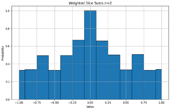
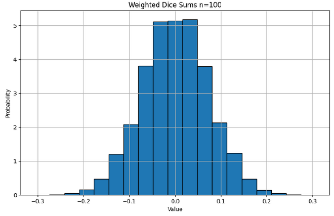
To more intuitively imagine a summation of random numbers, imagine rolling a dice with values \([-3,-2,-1,1,2,3]\), rolling it many times and taking the sum. If you roll it twice, the minimum and maximum total values you can get is is \([-6,6]\), and you are reasonably likely to get close to either extreme. However, if you roll the dice 100 times, the min and max total values you can get is \([-300, 300]\), however you are likely to get a score (total value) much closer to 0 as most your rolls cancel each other out. The variance proportionally reducing as the number of trials increases is a common and fundamental theme in statistics.
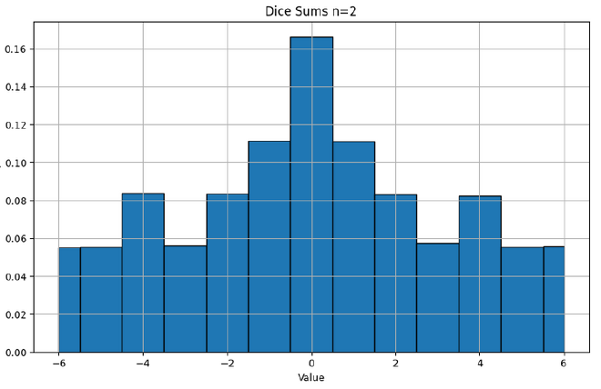
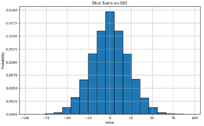
In our original equation for the angle, we divide by the magnitude of the vectors. The simplest analogy in our dice example is to divide by the maximum value achievable using the dice. Therefore, the full ‘game’ is to roll our dice \(n\) times, take the sum, then divide by \(3n\). I hope it is intuitive that as the number of rolls increases, more of our rolls as a proportion will be cancelled out by other rolls, and we are more likely to get a final weighted score that is closer to 0.
Angle Between Vectors#
Pairs#
Let’s now move to viewing the distribution of vectors. As a reminder, what the dot product does is:
$$ \mathbf{a} \cdot \mathbf{b} = a_1 b_1 + a_2 b_2 + \cdots + a_n b_n $$
And the equation for the angle is: $$ \cos{\theta} = \frac{\mathbf{a} \cdot \mathbf{b}}{|\mathbf{a}| |\mathbf{b}|} $$
To move from our dice game to the vector space, there are some subtle but not too impactful changes:
- we compute values in our sum by multiplying two random values from a and b together, instead of just rolling a singular die. (We are ultimately still just picking a random value, symmetrically distributed around 0)
- we divide by the magnitude of the vector, instead of the magnitude of the best possible rolls (the big picture is both scale the output of the sum to between [-1,1])
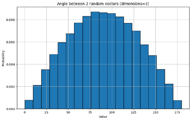
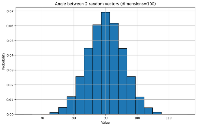
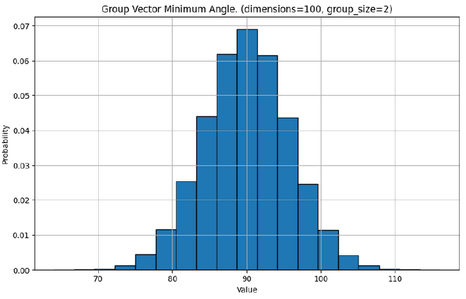
When we re-run the experiment using vectors, we unsurprisingly see similar behaviour as we scale up the number of dimensions
Larger Groups#
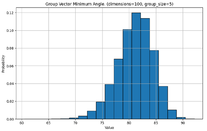
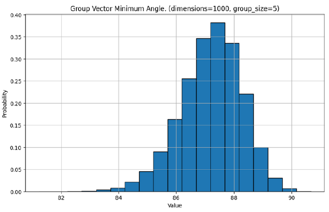
As pairs of vectors become increasingly more orthoganol as the number of dimensions increases, so do larger groups of vectors. Let’s look at the minimum angle between any two vectors in a group, for different size groups in different dimensions.
Application in Neural Networks#
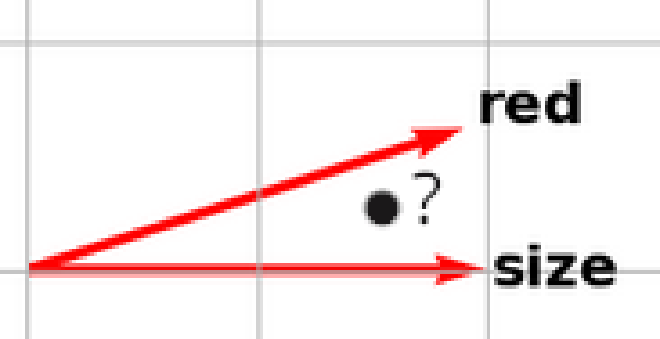
In modern LLMs, ideas (called features) are represented using vectors. For example, you might have a direction which represents size, so to represent the word ‘huge’, the LLM would assign it a vector that is strongly positive in the size direction. Superposition occurs when a single/similar direction in the model’s embedding space simultaneously represents multiple unrelated features, because the model has to pack many concepts into a limited number of dimensions. For example, if you look at the output of a neuron, it might have similar outputs when representing the idea of ‘size’ and ‘red’, despite those two ideas being quite distinct.
This is important in the field of mechanistic interpretability, which aims to try and reverse engineer neural networks into human understandable algorithms. In this field, superposition is a large barrier, because it makes it significantly harder to understand what a neuron activation means when it fires similarly for multiple different ideas (in this case, is the neuron firing because it is thinking about size, or redness?)
The goal of this section is to show why the number of near-orthagonal vectors in high dimensional spaces is often used as an explanation to why superposition appears in neural networks.
A Sense of Scale Using LLaMA 3#
The number of embedding dimensions, the number of dimensions used to encode a word, for modern LLMs tends to increase as the models overall size is scaled. For example, for LLaMA 3, the number of dimensions is:
| Number of Parameters | Number of Dimensions (word embedding) |
|---|---|
| 8 Billion | 4,096 |
| 70 Billion | 8,192 |
| 405 Billion | 16,384 |
Let’s take a look at the distribution of angles between any two random vectors in the embedding space of LLaMa 3’s largest model at 405 Billion Parameters.

Remember these experiments are just to give an intuition about the sparsity of vectors by looking at random vectors. When LLMs are trained, they can essentially ‘choose’ which vectors to use (associate with a given feature), meaning they can choose a packing which maximises orthagonality between many vectors. Alternatively, for a given required angle between all vectors, they can maximise the number of vectors they can use.
You have seen that the average fixed size group of vectors becomes more orthogonal to each other as the number of dimensions grows. In the same manner, the largest possible group you can make with a fixed required angle separation also grows as you increase the number of dimensions. For example, if you wanted to draw as many points on the edge of a circle as possible, where no two points are closer than 45 degrees, this would be less than the number of points you could draw on the surface of a sphere, where no two points are closer than 45 degrees.


In fact, the maximum size of a constrained group grows much faster than these graphs might indicate - it is known that the maximum number of near-orthogonal vectors scales exponentially with the number of dimensions.
The Kabatiansky-Levenshtein Bound gives an asymptotic formula for approximating this value (technically referred to as the maximal size of a spherical code in n dimensions). We can use this formula to illustrate the approximate shape and magnitude of the function relating the angle separation to the maximum group size for the dimensions used in LLaMA 3, however do not quote these values since the KL bound can become innaccurate for theta values close to 90 degrees.
| Minimum Angle Separation (degrees) | Dimensions | Approx. Max Number of Vectors |
|---|---|---|
| 88 | 16,384 | 10^20 |
| 85 | 16,384 | 10^99 |
| 80 | 16,384 | 10^322 |
Linking Feature Sparsity and Superposition#
As can be observed from the group size graphs earlier, if you increase the group size the average minimum angle between vectors decreases. Therefore, if you want to limit the probability of getting a certain level of similarity between vectors, there is a maximum limit to the group size you can use. In a similar vein, a crucial aspect of the KL bound formula is that the less orthogonality you have between your vectors - in other words the more similar your vectors are - the greater number of vectors you can pack into your space.
In deep learning, you want to be able to distinguish different feature vectors, so there is a limit to the allowable similarity between these vectors. If one imagines this allowable similarity as a limited resource, then there are two forces competing for it: a desire to increase the ‘group size’ (number of simultaneously active features) and a desire to increase the total number of vectors packed into the space (number of total representable features).
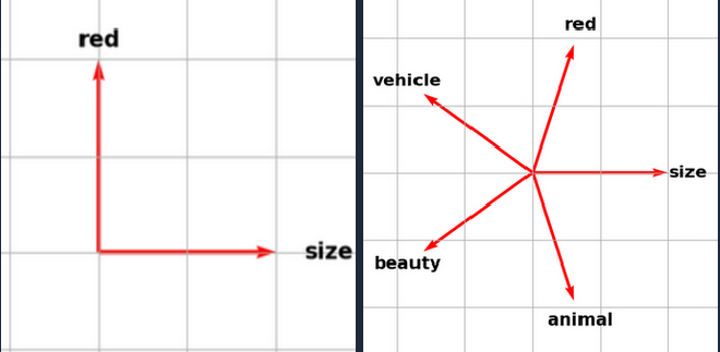
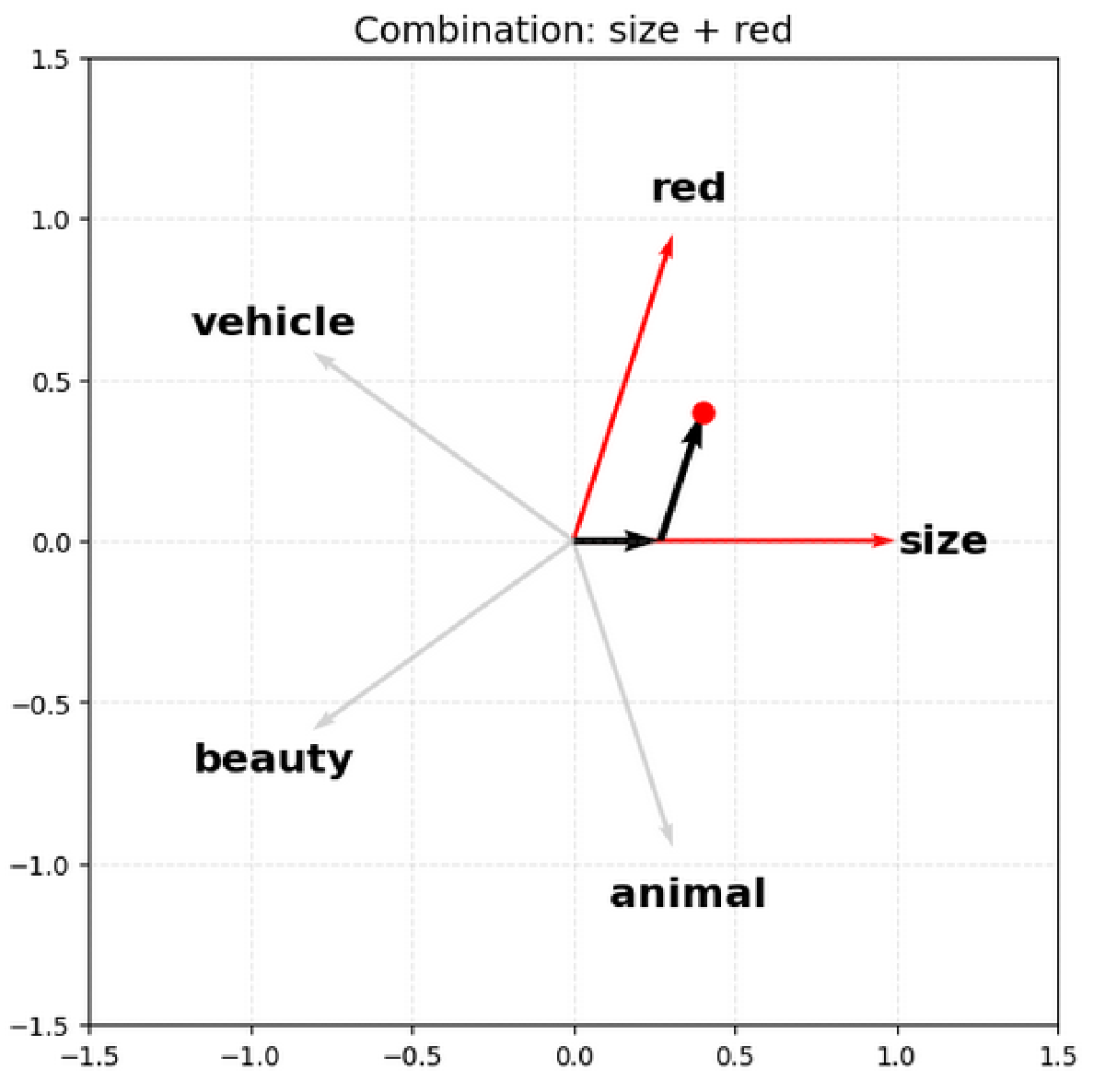
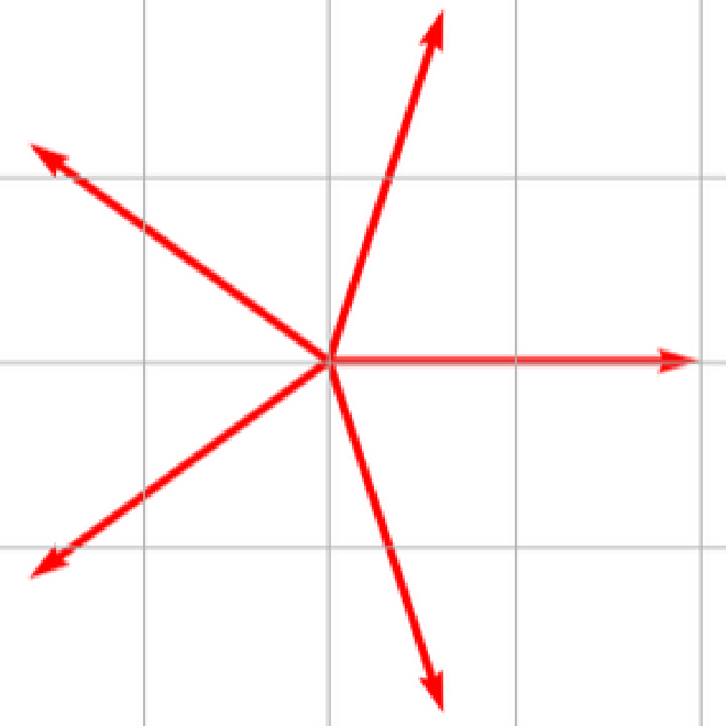
To further understand why you might not be able to have as many simultaneously firing feature vectors, consider that the output of the neurons will be a point in the embedding space. In the first case, with just ‘red’ and ‘size’, you can take any point and reverse engineer the vectors that were combined to make it. However, in the case where you have 5 total features and I show you a point that is a combination of two of them, you might struggle to confidently say for some points which vectors were ‘combined’ to get that point:


Therefore, the model has to learn a trade-off in its representation. For example, consider how the two models above might represent a car, or a ladybird.
| Total Known Features | Number of Active Features (group size) | Car Representation | Ladybird Representation |
|---|---|---|---|
| Size, Red | 2 | Fairly big, not very red | small, very red |
| Size, Red, Vehicle, Beauty, Animal | 1 | Definitely a vehicle | very red? |
In reality, the model doesn’t necessarily “choose” to only activate one feature, for example only representing a ladybird with “very red”. It will have detectors for ‘redness’, ‘size’ and ‘animal’, and if it was given a ladybird it would signal strongly for all of them. Instead, the model has to learn features that are both useful and don’t often appear all at once in the training dataset. For instance, if the training set contained many instances of ladybirds, the model learning 5 features may want to choose more specific and independent features. Alternatively, if there were far more instances of ladybirds than cars, another solution could be to remove the ‘vehicle’ feature completely, to better focus on the remaining, more important features.
This is why the sparsity of features is a useful predictor for the amount of superposition in a neural network. ‘Sparsity of features’ essentially means how often multiple features are active simultaneously as a proportion of the total identifiable features. Language can represent a vast array of ideas, but only a very small portion of those are present in a given word or sentence (or even LLM context window). This means the balance between the two fighting forces tips towards the total number of representable features, and as discussed before in order to be able to increase total features by packing more vectors into the space then you must accept more similar vectors for those features.
Greater similarity between feature vectors manifests as superposition, therefore language models like GPT pose a major challenge to interpretability researchers.
Conclusion and Further Reading#
High dimensional spaces can seem intimidating, however often this stems from trying to force yourself to think about problems geometrically, when they might be easier understood through another lens. Having a good conceptual understanding of such spaces can help understand modern neural networks, since modern applications are centred around transformers that use high dimensionality embeddings. These models ’think’ in high dimensionality spaces, so to understand the models it would seem useful to also understand the characteristics of how their thoughts are represented.
Understanding how the angle between vectors can affect feature representations is just the tip of the iceberg when it comes to understanding neural networks. I hope to gain a further grasp of other fundamental concepts that constrain and affect neural networks, especially when applied to mechanistic interpretability, and I would encourage others too to explore the topic. If you’re interested in mechanistic interpretability or AI safety more broadly, then Anthropic’s research is a great place to start:
- Toy Models of Superposition - an in-depth exploration of superposition (a great follow up from this post)
- Alignment Faking in Large Language Models - short and non-technical example of how modern LLM’s can strategically lie (the perfect introduction to AI safety)